Most explanations of contrastive learning hand you the math and move on. This is me writing down what actually clicked, after months of using it in a multimodal retrieval system, hitting walls, and slowly understanding why the method works the way it does.
I came to contrastive learning sideways. I was building a cross-modal retrieval system, images and text living in the same embedding space, queryable against each other, and kept running into this fundamental question: how do you get two completely different types of data to "mean" the same thing in vector space?
The answer kept pointing back to contrastive learning. So I went deeper, read the original papers, implemented pieces of it, and somewhere in that process, things clicked in a way they usually don't from just reading papers. This post is that understanding, written down.
The core idea
Here is the simplest version: you have an encoder. You want it to map semantically similar things close together and semantically different things far apart in embedding space. Contrastive learning is the training recipe that does this, without labels.
The trick is inventing your own supervision signal. Take an image. Apply two different random augmentations to it: crop, flip, color jitter. Now you have two views of the same image. They look different but they're semantically the same thing. Those are your positives. Everything else in the batch is a negative.
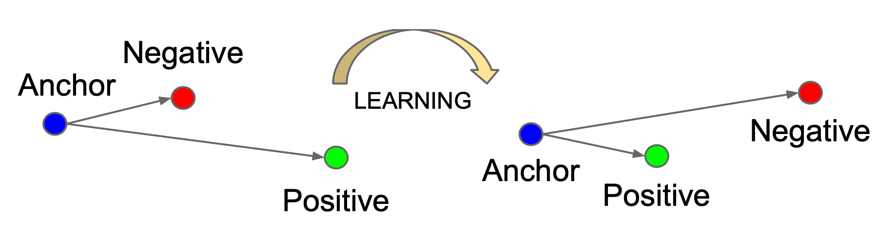
Fig 1. Triplet mapping concept: pulling the anchor close to positive views while pushing the negative samples beyond a configured margin (Schroff et al., 2015).
Train the encoder to score positive pairs higher than negative pairs, and eventually it learns to embed images by their semantic content rather than low-level pixel statistics. The augmentations define what "same" means, and by extension, what the encoder should be invariant to.
The loss function: InfoNCE
The loss that made all of this work at scale is InfoNCE. For a batch of N samples, each with one positive:
where z_i = f(x_i) are the projected embeddings and \tau is a temperature hyperparameter.
The easiest way to read this: it's an N-way classification problem. For each anchor, identify which sample in the batch is the positive. The denominator sums over all N samples, so the model gets penalized whenever a negative ends up with high similarity to the anchor.
Temperature is the hyperparameter I spent the most time understanding. The standard framing ("low temperature = more confident, high temperature = more random") is technically true but doesn't tell you what it's actually doing. What it's doing is controlling which negatives contribute gradient. Low temperature makes the model hyperfocus on whoever is closest to the anchor and getting it wrong. High temperature distributes attention across all negatives.
SimCLR: the clean baseline
SimCLR (Chen et al., 2020) is the method that made contrastive learning the dominant paradigm for self-supervised image representation. Its contribution wasn't a new loss function; it was an unusually systematic study of what actually matters in the pipeline.
The projection head detail is one of those things that seems like a footnote but isn't. When I first read the paper I glossed over it. Then I understood what it means: the projection head appears to throw away information that helps the contrastive objective but hurts downstream tasks. By training with it and then removing it, you get an encoder that builds richer representations than it would if the loss hit it directly. It's doing a kind of information routing that wasn't designed in, it just emerged.
The other finding that stuck with me: augmentation composition matters far more than architecture. Crop + color jitter is not just "a good combination"; it's almost necessary. Cropping forces the model to recognize parts as belonging to the whole. Color jitter removes an easy shortcut (matching by histogram) and forces it to learn shape. Remove either one and representations degrade measurably.
MoCo: decoupling negatives from batch size
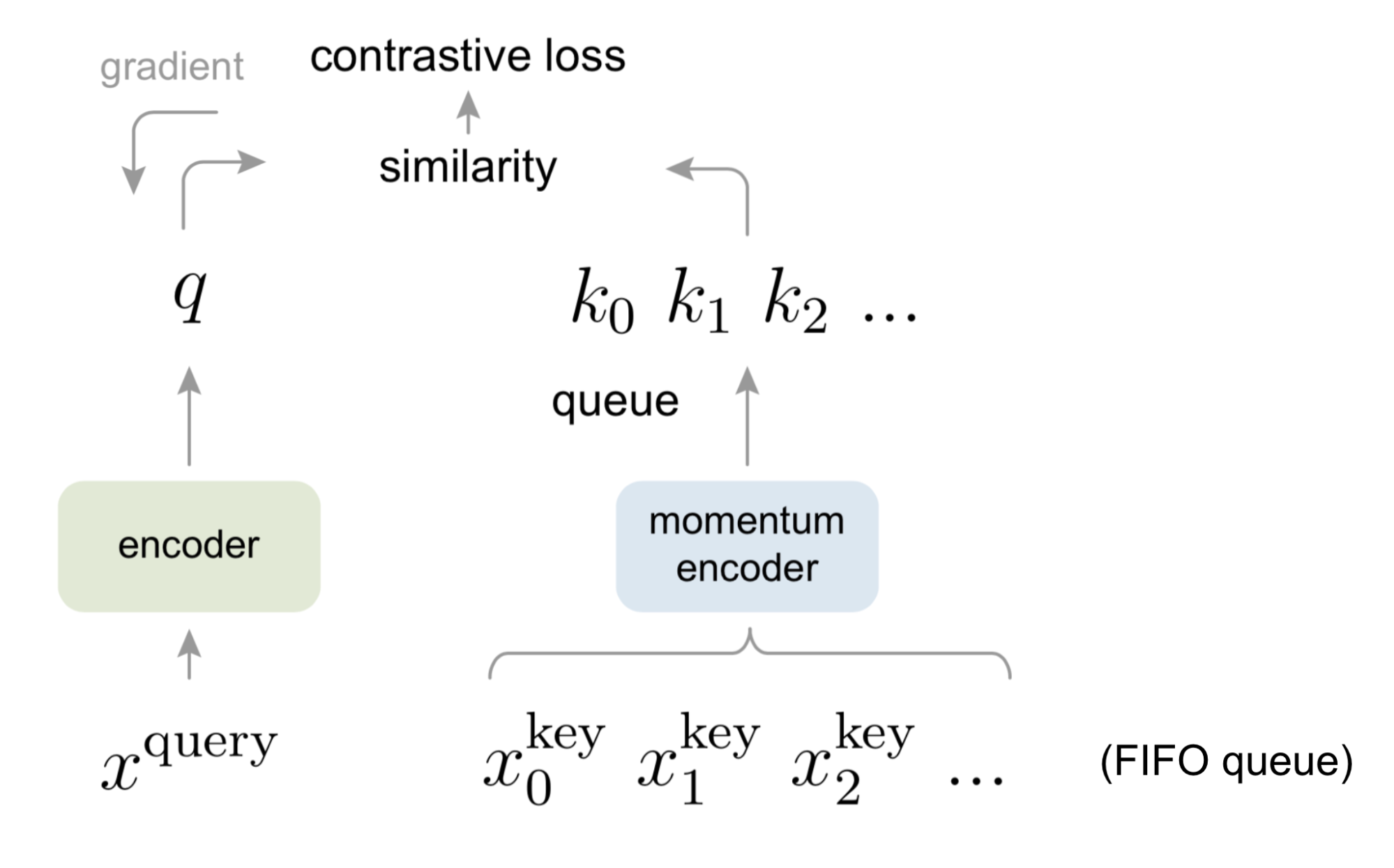
Fig 2. MoCo workflow: query representations are checked against a dynamic FIFO queue of recent keys encoded by a slowly drifting momentum encoder (He et al., 2019).
Momentum Contrast (He et al., 2020) kept the contrastive objective but changed where negatives come from. Instead of the current batch, MoCo maintains a queue of encoded keys from recent batches. This lets you have 65k negatives regardless of batch size.
The EMA update is what makes the queue coherent. If the key encoder updated at the same speed as the query encoder, old keys in the queue would be stale, encoded by a meaningfully different model. Slow EMA keeps the key encoder drifting gradually, so the queue stays approximately from the same distribution. MoCo v2 added SimCLR's projection head and stronger augmentation, closing most of the gap with SimCLR while using a fraction of the batch size.
BYOL: no negatives needed
BYOL (Grill et al., 2020) is the one that really surprised me when I first understood it. It removed negatives entirely. By any intuition about what contrastive learning is doing, this should not work.
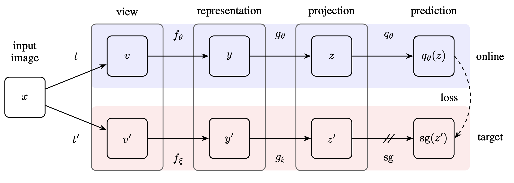
Fig 3. BYOL architecture: the online network uses a predictor to match target features, while target network weights are slowly updated as an EMA of the online parameters (Grill et al., 2020).
The loss is the negative cosine similarity between the online network's prediction of one view and the target network's projection of another view:
No negatives. The loss is minimized when the prediction matches the target projection.
The obvious failure mode is collapse: if the encoder outputs the same constant vector for every input, the loss is zero. But BYOL doesn't collapse. The honest answer to why is: we don't fully know. The EMA target creates a consistent but always slightly ahead bootstrap signal. The predictor creates an asymmetry that makes the trivial solution unstable. Batch normalization in the projector implicitly carries batch-level statistics that act as a soft negative signal.
Whether these explanations are complete is still debated. What's not debated is that BYOL works; it matches SimCLR on ImageNet linear evaluation while being far less sensitive to batch size.
Barlow Twins: a different objective entirely
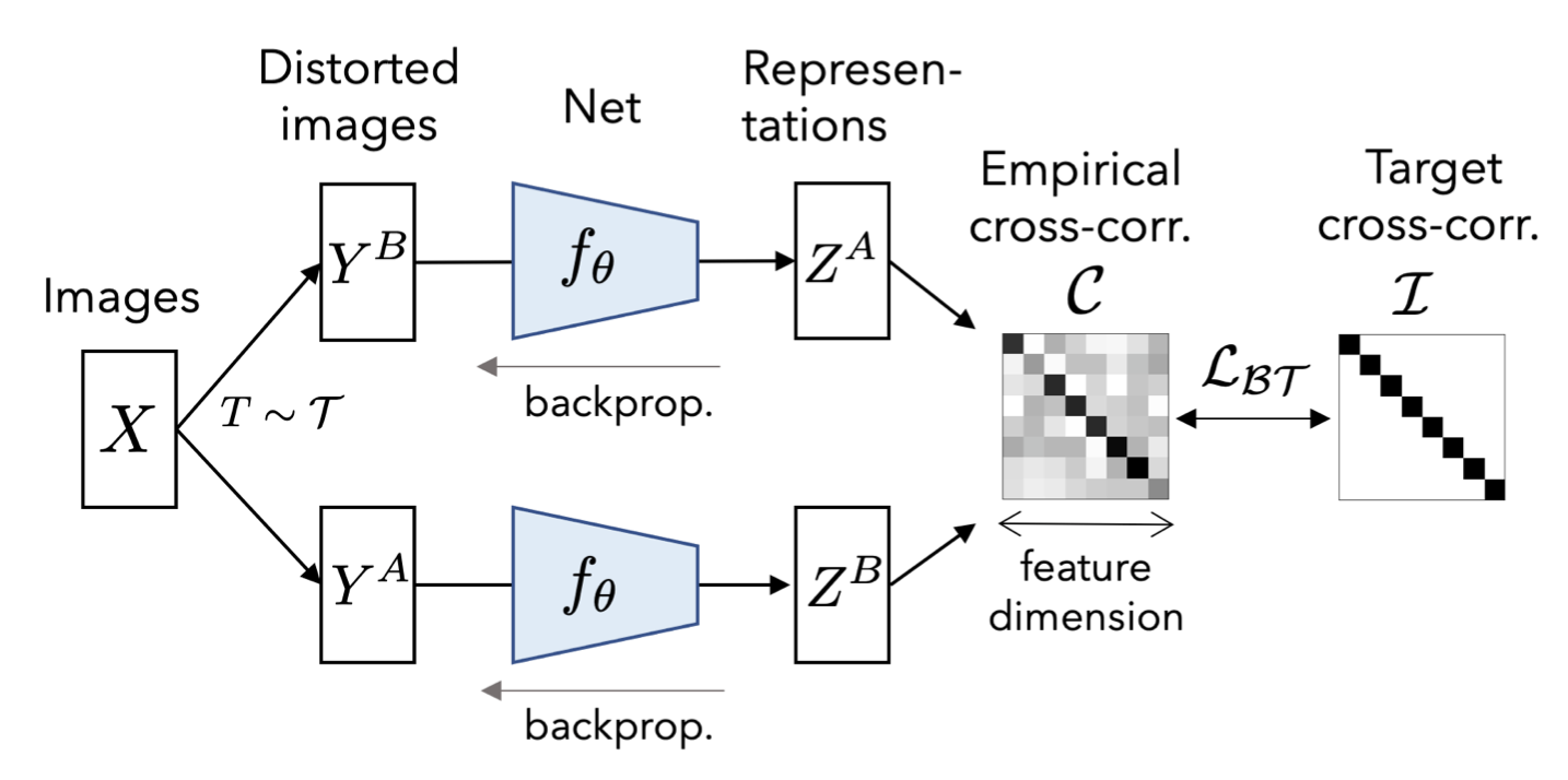
Fig 4. Barlow Twins: feeds twin augmented views to optimize a cross-correlation matrix toward the identity matrix, reducing representational redundancy (Zbontar et al., 2021).
Barlow Twins (Zbontar et al., 2021) takes a different angle. Instead of pulling positives together and pushing negatives apart, the objective is to make the cross-correlation matrix of the embeddings close to the identity matrix:
$$\text{where } C_{ij} = \frac{\sum_b z^A_{b,i} \cdot z^B_{b,j}}{\sqrt{\sum_b (z^A_{b,i})^2} \sqrt{\sum_b (z^B_{b,j})^2}}$$
Invariance term: diagonal elements should be 1. Each dimension of the embedding should be maximally correlated between the two views of the same image.
Redundancy reduction term: off-diagonal elements should be 0. Different embedding dimensions should be decorrelated from each other, meaning each dimension captures independent information.
What I find elegant about this is the redundancy reduction term. Each embedding dimension is forced to carry non-overlapping information. This is essentially a whitening objective: the representation is maximally informative because no two dimensions are encoding the same thing. It works with small batches, scales well with embedding dimension, and requires no momentum encoder.
CLIP: across modalities
CLIP (Radford et al., 2021) is what started my real interest in this area, because it's where contrastive learning became the foundation for something I was actually building.
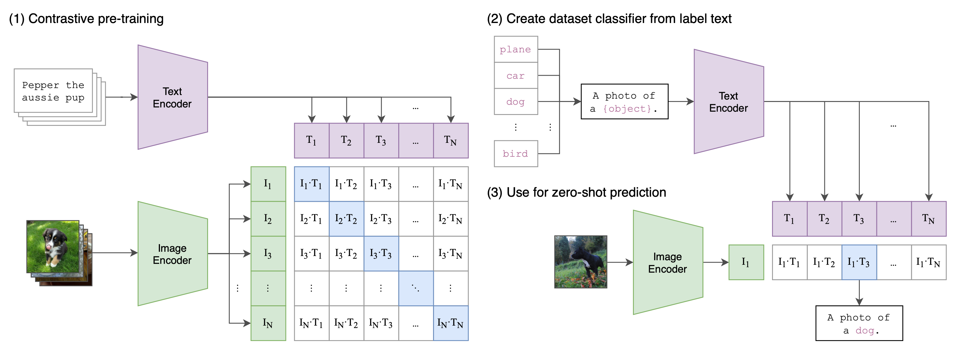
Fig 5. CLIP joint pretraining: optimizes a symmetric cross-entropy loss over a dense similarity matrix to align matching text-image pairs in a shared space (Radford et al., 2021).
What CLIP showed me about contrastive learning: the framework is not specific to vision. The only requirement is two views that share semantic content. Images and their captions share semantic content. Audio and transcripts. Code and documentation. The framework generalizes to any modality pair where you have co-occurring signal.
The training objective is symmetric InfoNCE over a batch of N (image, text) pairs. Each image should be closer to its paired text than to the other N-1 texts, and vice versa. It optimizes a joint loss that aligns matching pairs in a shared space:
When I moved to SigLIP for my retrieval system, the core idea was the same as CLIP but with sigmoid loss instead of softmax. The practical difference: SigLIP doesn't require the full batch sum in the denominator, so it's less sensitive to batch composition and scales better to large batches with many negatives. For retrieval tasks where you want fine-grained matching, it tends to produce better-calibrated similarity scores.
Hard negative mining
The quality of negatives determines the quality of your representations. Easy negatives (images that are obviously different from the anchor) provide near-zero gradient once the model has learned basic structure. The real learning signal comes from hard negatives: images that are superficially similar but semantically different.
There are a few main ways to get them:
- In-batch hard negatives: Within a batch, upweight the negatives with the highest similarity to the anchor rather than treating all negatives equally. Simple to implement, but heavily limited by batch diversity.
- Memory bank / queue: Store encoded representations from previous iterations. MoCo's queue is the classic implementation here, allowing you to select hard negatives from a pool much larger than any single batch.
- Synthetic hard negatives: Mix embeddings in latent space to create representations that sit directly near the decision boundary. This is more aggressive, but carries a real risk of creating false negatives: synthetic samples that happen to actually be semantically similar to the anchor.
How these methods compare
| Method | Negatives? | Momentum enc.? | Key constraint |
|---|---|---|---|
| SimCLR | In-batch | No | Large batch (4k+) |
| MoCo v2 | Queue | Yes | Queue coherence via EMA |
| BYOL | None | Yes (target net) | Predictor + EMA to prevent collapse |
| Barlow Twins | None | No | Large embedding dim helps |
| CLIP / SigLIP | Cross-modal in-batch | No | Needs matched pairs at scale |
What the representations actually learn
The standard benchmark is linear evaluation: freeze the encoder, train a linear classifier on top, report accuracy. It tests how linearly separable the embedding space is. On ImageNet with ResNet-50, the best contrastive methods reach 70–75% top-1, vs ~76% for fully supervised training. The gap has closed a lot since 2020.
The more interesting question is transfer. Contrastive representations consistently outperform supervised representations when you move to tasks that differ from the pretraining domain, such as medical imaging, remote sensing, and scientific data. The contrastive objective forces the encoder to build more general structure because there's no fixed label set to overfit to. It has to learn what's common across augmented views of the same image, which tends to be semantic content rather than dataset-specific statistics.
One thing I've noticed in practice: contrastive embeddings have more internal structure than supervised ones. Related classes cluster together in ways that supervised training doesn't enforce. When I'm doing cross-modal retrieval and something goes wrong, it's almost never that the embedding space is random; it's usually that the boundary between two similar-looking categories is too soft. That's a property of the training distribution, not a failure of the method.
Practical notes
A few things worth knowing if you are actually running these methods and not just reading about them:
Projection head nonlinearity matters more than dimension. The ReLU in the hidden layer of the projection MLP makes a measurable difference. Output dimension anywhere from 128 to 2048 works similarly. Don't spend much time tuning the dimension.
Training needs to run longer than supervised training to converge. 100-epoch evaluations consistently underestimate final performance. Plan for 200+ epochs minimum on ImageNet-scale data.
If you're working outside natural images (medical imaging, satellite data, scientific microscopy), treat the augmentation policy as a first-class design decision, not a default setting. What should be invariant in your domain is not what was invariant in ImageNet pretraining. Aggressive color jitter and random cropping can destroy exactly the information you're trying to preserve.
For multimodal settings specifically: the quality of your matched pairs matters as much as the training recipe. Noisy correspondences (captions that don't describe the image, misaligned audio/video) corrupt the positive signal more than any hyperparameter choice will compensate for.
Where things are now
The core methods are mature at this point. SimCLR, MoCo, BYOL, Barlow Twins, CLIP, and SigLIP are stable, well-understood industry baselines. But the self-supervised landscape has expanded into two major directions that shift away from traditional contrastive learning:
1. Joint Embedding Predictive Architectures (JEPA)
Yann LeCun's team at Meta has pushed heavily for JEPA (such as I-JEPA and V-JEPA) as a way to avoid both the false-negative problem of contrastive learning and the pixel-reconstruction overhead of Masked Autoencoders (MAE). Instead of pulling augmented views together, JEPA works by masking regions of an input (like an image or video) and training a predictor to predict the abstract representation (embedding) of the missing region from the context region. It learns a world model in latent space, stripping out pixel-level noise to focus entirely on high-level semantic structures.
2. The shift to generative, autoregressive pretraining
In multimodal systems, we've seen a massive transition. While contrastive dual-encoders (like CLIP and SigLIP) remain the standard for heavy retrieval and embedding search, generative multimodal foundation models (like LLaMA-Vision, Chameleon, and Gemini) have largely taken over reasoning and generative tasks. Instead of pre-aligning distinct image and text embedding spaces via contrastive losses, these architectures project visual patches directly into LLM token spaces, pretraining end-to-end on unified autoregressive next-token prediction over interleaved image-text streams.
The contrastive framework turns out to be an incredibly successful chapter of self-supervised learning. It taught us how to structure vector spaces without labels, how to define inductive bias through data augmentations, and how to prevent representation collapse. Whether it remains the dominant pretraining paradigm or serves as the retrieval-specialized backbone for generative giants, the core lessons of contrastive representation learning remain the foundation of how we build modern AI systems.